Implements multi-dimensional Polynomial Chaos Expansion (PCE) for spectral surrogate modeling.
More...
|
| | PolynomialExpansion ()=default |
| |
| void | set (size_t dimension, size_t totalDegree, const Eigen::VectorXd &p1, const Eigen::VectorXd &p2, double q=1.0) |
| |
| void | fit (const Eigen::Ref< const Eigen::MatrixXd > &samples, const Eigen::Ref< const Eigen::VectorXd > &values) |
| |
| double | getAnalyticalMean () const |
| |
| double | getAnalyticalVariance () const |
| |
| Eigen::VectorXd | getSobolMainIndices () const |
| |
| Eigen::VectorXd | predictBatch (const Eigen::Ref< const Eigen::MatrixXd > &X) const |
| |
| std::pair< double, double > | predict (const Eigen::Ref< const Eigen::VectorXd > &x) const |
| |
| std::pair< double, double > | predictWithObs (const Eigen::Ref< const Eigen::VectorXd > &x, const double &yObs) const |
| |
| std::pair< double, double > | predictLOO (const size_t &i) const |
| |
| Eigen::VectorXd | computeBasisRow (const Eigen::Ref< const Eigen::VectorXd > &x) const |
| |
| void | save (const std::string &filename) const |
| |
| void | load (const std::string &filename) |
| |
| size_t | getNumBasisFunctions () const |
| |
| void | project (const std::function< double(const Eigen::VectorXd &)> &model, int pointsPerDim) |
| |
Implements multi-dimensional Polynomial Chaos Expansion (PCE) for spectral surrogate modeling.
- Template Parameters
-
Mathematical Foundations
Polynomial Chaos Expansion represents a stochastic model output \(Y = f(\mathbf{X})\) as a spectral expansion of multivariate orthogonal polynomials mapping canonical variables \(\boldsymbol{\xi}\):
\[ Y \approx \sum_{j=0}^{P-1} c_j \Psi_j(\boldsymbol{\xi}) \]
The multivariate polynomials \(\Psi_j(\boldsymbol{\xi})\) are tensor products of univariate orthogonal polynomials:
\[ \Psi_j(\boldsymbol{\xi}) = \prod_{i=1}^d \psi_{\alpha_i^{(j)}}(\xi_i) \]
where \(\boldsymbol{\alpha}^{(j)} = (\alpha_1^{(j)}, \dots, \alpha_d^{(j)})\) is the multi-index of polynomial degrees.
Uni-dimensional orthogonal bases satisfy:
\[ \int_{\Omega} \psi_k(x) \psi_l(x) w(x) dx = \gamma_k \delta_{kl} \]
where \(w(x)\) is the probability density function (PDF) weight of the canonical distribution.
Implementation Algorithms
- Canonical Mapping: Physical samples \(\mathbf{x}\) are mapped to canonical space \(\boldsymbol{\xi}\) using the basis-specific mappings (
mapToCanonical).
- Design Matrix Construction: Computes the regression matrix \(\mathbf{A} \in \mathbb{R}^{N \times P}\) where:
\[ A_{ij} = \Psi_j(\boldsymbol{\xi}^{(i)}) \]
- Ordinary Least Squares (OLS) Regression: The expansion coefficients \(\mathbf{c}\) are found by solving the linear least-squares problem \(\mathbf{A}\mathbf{c} \approx \mathbf{y}\):
\[ \mathbf{c} = \left(\mathbf{A}^T \mathbf{A}\right)^{-1} \mathbf{A}^T \mathbf{y} \]
We solve this system robustly using Column-Pivoted Householder QR decomposition (ColPivHouseholderQR).
Constraints & Invariants
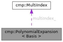
- Sample Size: The number of samples \(N\) must satisfy \(N > P\) (where \(P = \text{multiIndex\_.size()}\)) to avoid an underdetermined system and severe overfitting.
- Parameter Ranges: Bounding parameter vectors (e.g., mean/standard deviation or lower/upper bounds) must match the dimensionality of the input space.