MCMC thinning
The following blog post analyses the effect of subsampling a Markov chain. Subsampling (or thinning) is a common operation that consists of discarding N samples before saving the next one when sampling an MCMC (Markov Chain Monte Carlo). This is done for two main reasons. First and foremost, it saves memory by reducing the number of samples that have to be analyzed. Moreover; even with a perfect acceptance rate, samples will always be correlated. To ensure independence between samples, they have to be “thinned”; between two saved samples, some samples compatible with the correlation length need to be discarded. Such samples will be then used to construct statistics or estimators so it is natural to ask if subsampling is necessary. If the answer is yes, how much? We will try to answer this question by looking at the quality of the mean estimator as a function of the subsampling ratio.
\[\newcommand{\muh}{\hat{\mu}} \newcommand{\summ}[3]{\displaystyle \sum_{#1=#2}^{#3}} \newcommand{\dd}{\text{d}} \newcommand{\qt}{\tilde{q}} \newcommand{\var}{\text{var}} \newcommand{\cov}{\text{cov}} \newcommand{\vh}{\hat{V}}\]
Assume that we have \(n\) samples \(\{q_i\}_{i<n}\) taken from the realization of a Markov chain that has converged to the stationary distribution \(p(q)\). The expected value of the distribution will be estimated using the sample average in the following way
\[\begin{equation} \left. \begin{aligned} & \mu = E(q) = \int_\mathcal{Q} q \ p(q) \, \dd q \; , \\ & \muh = \dfrac{1}{n} \summ{i}{1}{n} q_i \; . \end{aligned} \right. \end{equation}\]Even if the samples are not independent, the expected value of this estimator will be, because of the linearity of the expectation operator:
\[\begin{equation} E(\muh) = \dfrac{1}{n}\summ{i}{1}{n} E(q_i) = \mu \; . \end{equation}\]Defining \(\qt_i = q_i - \mu\), we can compute the variance in the following way:
\[\begin{equation} \var(\muh) = E\left( (\muh -\mu)^2\right) = E\left( \dfrac{1}{n^2} \summ{i}{1}{n} \qt_i \summ{j}{1}{n} \qt_j\right) \; . \end{equation}\]The product between the sample sum can be decomposed by noting that
\[\begin{equation} \left. \begin{aligned} (\qt_1 + \qt_2 + \ldots+ \qt_n)& (\qt_1 + \qt_2 + \ldots + \qt_n)= \\ & \qt_1^2 + \qt_2^2 + \ldots + \qt_n^2 \\ & +2\qt_1 \qt_2 + \ldots + 2\qt_1 \qt_n \\ &+ \ldots + 2 \qt_2 \qt_n \\ & + \ldots \end{aligned} \right. \end{equation}\]Hence,
\[\begin{equation} \var(\muh) = \dfrac{1}{n^2} E\left( \summ{i}{1}{n} \qt_i^2 + 2 \summ{i}{1}{n-1}\summ{j}{i+1}{n} \qt_i\qt_j\right) = \dfrac{1}{n^2} \left( \summ{i}{1}{n} E(\qt_i^2) + 2 \summ{i}{1}{n-1}\summ{j}{i+1}{n} E(\qt_i\qt_j) \right) \; . \end{equation}\]And finally,
\[\begin{equation} \var(\muh) = \dfrac{\sigma^2}{n} + \dfrac{2}{n^2} \summ{i}{1}{n-1}\summ{j}{i+1}{n} \cov(\qt_i,\qt_j) \; . \label{eq:var} \end{equation}\]We now assume an exponential decay of the covariance between samples,
\[\begin{equation} \cov(\qt_i,\qt_j) = \sigma^2 \ \exp\left( -\dfrac{|i-j|}{L}\right) \; , \label{eq:cov} \end{equation}\]where the factor \(\sigma^2\) ensures that when \(i=j\) we retrieve the correct variance and \(L\) is an appropriate correlation length scale. We denote \(k=\mid i-j\mid\) as the lag. Substituting Eq. \ref{eq:cov} into Eq. \ref{eq:var} yields
\[\begin{equation} \left. \begin{aligned} \var(\muh) & = \dfrac{\sigma^2}{n} + \dfrac{2}{n^2} \summ{i}{1}{n-1}\summ{k}{1}{n} \exp\left( -\dfrac{k}{L}\right) \\ & = \dfrac{\sigma^2}{n} \left( 1+ 2\frac{n-1}{n} \summ{k}{1}{n} \exp\left( -\dfrac{k}{L}\right) \right)\; . \end{aligned} \right. \end{equation}\]To rewrite the last term we have used the fact that the term inside the exponential does not depend on the running index i. Now we introduce the thinning parameter s which can be an integer value between 1 and n-1. It corresponds to how much the chain is thinned, i.e. we retain 1 every s samples. As an example, when s is equal to 1 we do not discard any sample and we immediately save the next sample. When s is equal to n-1 we accept the first sample and then discard all the subsequent n-1 samples, remaining with just one sample. For the sake of brevity, we also call \(\tilde{n}=\frac{n/s-1}{n/s}\)
\[\begin{equation} \var(\muh) = \dfrac{\sigma^2}{n/s} \left( 1+ 2 \tilde{n}\summ{k}{1}{n/s} \exp\left( -\dfrac{k s}{L}\right) \right)\; . \end{equation}\]The sum evaluates to,
\[\begin{equation} \summ{k}{1}{n/s} \exp\left( -\dfrac{k s}{L}\right) = \dfrac{e^{-n/L}\left( e^{n/L}-1\right)}{e^{s/L}-1} \; . \end{equation}\]We now compute the ratio between the sample variance and \(L\frac{\sigma^2}{n}\) which has the dimensionality of variance and does not depend on the thinning parameter, \(s\),
\[\begin{equation} \dfrac{\var(\muh)}{L \frac{\sigma^2}{n}} = \frac{s}{L} \left( 1 - 2 \tilde{n} \dfrac{1-e^{-n/L}}{1-e^{s/L}} \right)\; . \end{equation}\]We now proceed by looking at the last equation as a function of \(x=s/L\) (which compares the amount of skipping to the correlation length), we call \(c = \tilde{n} \left(1-e^{-n/L} \right)\),
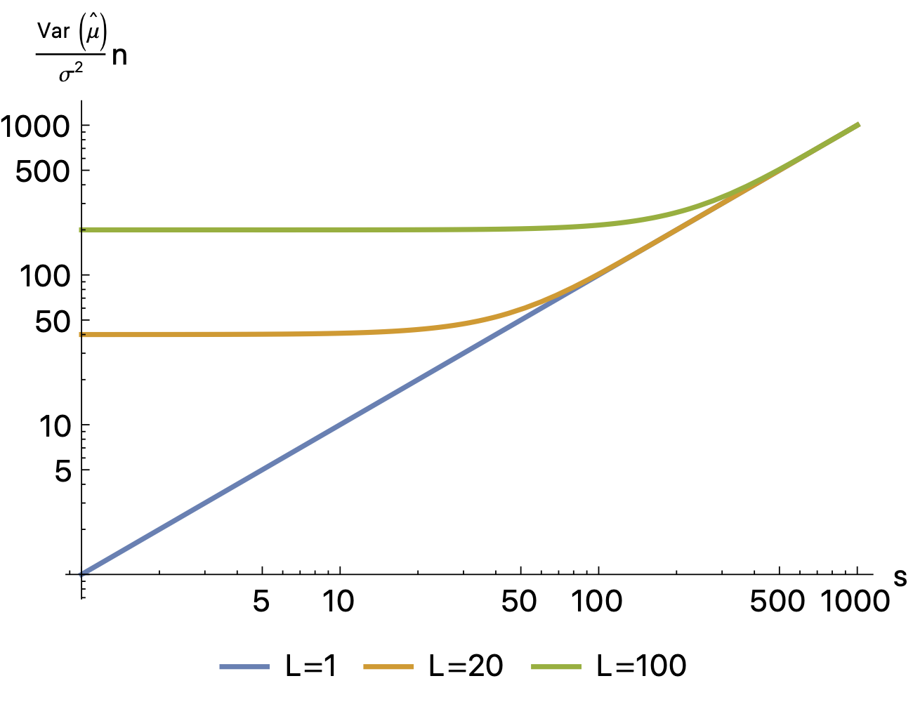
\[\begin{equation} f(x) = x \left(1 - 2\dfrac{c}{1-e^x} \right) \; . \end{equation}\]The parameter c is limited by 0 when \(n \rightarrow 0\) or \(L \rightarrow \infty\) and 1 when \(n \rightarrow \infty\) or \(L \rightarrow 0\) (assuming that we still accept a sufficient number of samples so that \(\tilde{n}=1\), otherwise we get a lower value). We call these limits the fully correlated and uncorrelated limits, respectively. We can show that this function is always monotone (for values of c in the range [0,1]). This means that thinning has no beneficial effect on the quality of the estimator. The following graph shows the increase in variance caused by thinning

On the one hand, subsampling always has a detrimental effect on the quality of the estimator. On the other hand, it is possible to see that this effect is negligible up to \(s/L \approx 1\), meaning that we can still subsample without any negative effect and reduce the dimension of the analyzed samples.
This has a positive effect as we have to analyze and store fewer samples.